Classification with Keras and the Iris Dataset
The Dataset
The Iris Dataset is a small dataset commonly used to test classification models. If you haven’t seen it before, you’ll see it again. The dataset consists of 150 samples of measurements taken from 3 species of Iris flowers. It can be found here.
The reasons for using this dataset are two-fold, it’s a small dataset with easy to understand class distinctions and it is relatively simple to train a neural network to recognize those classes.
sepal_length, sepal_width, petal_length, petal_width, species
5.1, 3.5, 1.4, 0.2, Iris-setosa
4.9, 3.0, 1.4, 0.2, Iris-setosa
4.7, 3.2, 1.3, 0.2, Iris-setosa
4.6, 3.1, 1.5, 0.2, Iris-setosa
5.0, 3.6, 1.4, 0.2, Iris-setosa
5.4, 3.9, 1.7, 0.4, Iris-setosa
4.6, 3.4, 1.4, 0.3, Iris-setosa
5.0, 3.4, 1.5, 0.2, Iris-setosa
4.4, 2.9, 1.4, 0.2, Iris-setosa
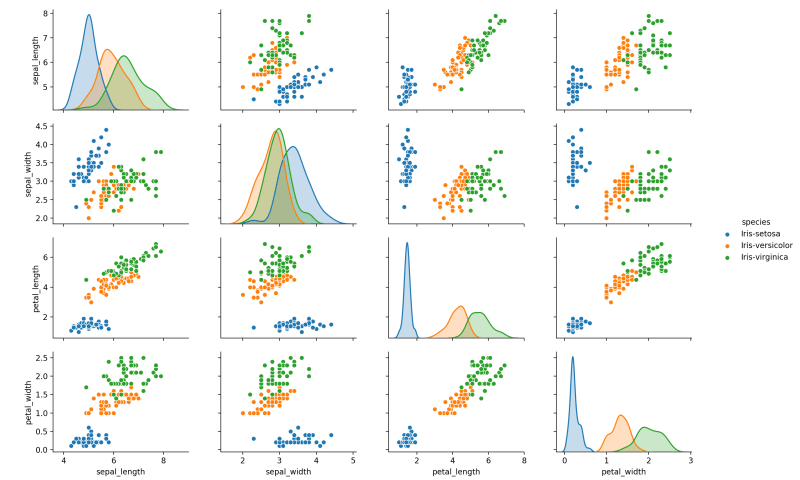
4.9, 3.1, 1.5, 0.1, Iris-setosaA great way to explore the distribution and possible relationships in the data is by using a scatter matrix. Seaborn is an excellent library for this purpose:
import seaborn
import matplotlib.pyplot as plt
dataframe = pandas.read_csv("iris.data", names=['sepal_length', 'sepal_width', 'petal_length', 'petal_width', 'species'])
seaborn.pairplot(dataframe, hue="species")
plt.show()
First we import and split the data into input and output:
import pandas

# Load the Iris dataset
dataframe = pandas.read_csv("iris.data", header=None)
dataset = dataframe.values

# Split into input (first four columns) and output (last column)
X = dataset[:,0:4]
Y = dataset[:,4]
One Hot Encoding the Output
Since neural networks aren’t designed with the use of human-friendly class labels in mind, we need to encode the species into numeric values. On top of that, we don’t want the model to generate a single output. For one, this type of encoding implies that classes whose labels happen to be encoded into adjacent integers are somehow related.
To prevent this we use one-hot encoding. The output is transformed from a single value into one feature (column) for each possible output class where the appropriate class has a value of 1 (hot) and all others are 0. This way, we can train the model to classify observations without any implied relationships between classes.
from keras.utils import np_utils
from sklearn.preprocessing import LabelEncoder

# Encode classes as integers
encoder = LabelEncoder()
encoder.fit(Y)
encoded_Y = encoder.transform(Y)

# One hot encode integer labels
one_hot_Y = np_utils.to_categorical(encoded_Y)
K-Fold Cross-Validation
We’re going to use k-fold cross-validation because it’s a good way to test whether a model performs well on unseen data. Typically, you use a portion of data that a model wasn’t trained on to validate its performance. K-fold cross validation takes this a step further by essentially using the entire dataset as a validation set. This is accomplished by splitting the data into k number of folds where one is held out as the validation dataset and the remaining as the training dataset. The validation process creates a new model for each fold and therefore by the end of the entire cross-validation, the entire dataset has been tested against. The average performance over all folds gives a realistic idea of how the model would perform on new data.
from sklearn.model_selection import KFold

# Create the k-folds cross-validator
num_folds = 5
kfold = KFold(n_splits=num_folds, shuffle=True)

from keras.models import Sequential
from keras.layers import Dense
Creating and Cross-Validating the Model
The architecture for this model is pretty simple:
def get_model():
    # Create model
    model = Sequential()
    model.add(Dense(10, input_dim=4))
    model.add(Dense(3, activation='softmax'))

    # Compile model
    model.compile(loss='categorical_crossentropy', optimizer='adam', metrics=['accuracy'])

    return model
There is a single hidden layer with 4 inputs (the four input data columns) connected to the output layer which contains three neurons.
We use softmax as the output activation function on the output layer because it means the output neurons will all equal 1 allowing us to interpret the output of the model as probabilities for each class. This choice is important to understand because the network has no understanding about what it is modeling. We are choosing activation functions and loss functions based on what we as humans want the model to output.
The loss function for training, Categorical Cross-entropy, is just a fancy way of saying that the model will be trained to generate a single high output (the class).
To implement the cross-validatie loop through the folds in the k-fold we created above and train a new model and print out some basic statistics for each:
num_epochs = 20
train_scores = []
test_scores = []
fold_index = 1

# Train model for each fold
for train, test in kfold.split(X, one_hot_Y):

    # Create model
    model = get_model()

    # Fit the model
    history = model.fit(
        X[train],
        one_hot_Y[train],
        validation_data=(X[test], one_hot_Y[test]),
        epochs=num_epochs,
        batch_size=5,
        verbose=0
    )

    # Preserve the history and print out some basic stats
    train_scores.append(history.history['acc'])
    test_scores.append(history.history['val_acc'])
    print("Fold %d:" % fold_index)
    print("Training accuracy: %.2f%%" % (history.history['acc'][-1]*100))
    print("Testing accuracy: %.2f%%" % (history.history['val_acc'][-1]*100))

    fold_index += 1
Note that we’re preserving the history of each training run for use in the next section.
Plotting Cross-Validation Performance
Visualizing the performance of a model during training is an important tool for developing your models. Calculating the final accuracy of the model against the training and validation data is important but it gives you no insight into how or if that number can be improved.
Because we collected the training history data for each fold in our cross-validation loop, plotting their averages and distribution is pretty straightforward:
import matplotlib.pyplot as plt

# Set up the plot
plt.figure()
plt.title('Cross-Validation Performance')
plt.ylim(0.2, 1.01)
plt.xlim(0, num_epochs-1)
plt.xlabel("Epoch")
plt.ylabel("Score")
plt.grid()

import numpy as np

# Calculate mean and distribution of training history
train_scores_mean = np.mean(train_scores, axis=0)
train_scores_std = np.std(train_scores, axis=0)
test_scores_mean = np.mean(test_scores, axis=0)
test_scores_std = np.std(test_scores, axis=0)

# Plot the average scores
plt.plot(
    train_scores_mean,
    '-',
    color="b",
    label="Training score"
)
plt.plot(
    test_scores_mean,
    '-',
    color="g",
    label="Cross-validation score"
)

# Plot a shaded area to represent the score distribution
epochs = list(range(num_epochs))
plt.fill_between(
    epochs,
    train_scores_mean - train_scores_std,
    train_scores_mean + train_scores_std,
    alpha=0.1,
    color="b"
)
plt.fill_between(
    epochs,
    test_scores_mean - test_scores_std,
    test_scores_mean + test_scores_std,
    alpha=0.1,
    color="g"
)

plt.legend(loc="lower right")
plt.show()
The blue line and shading represents the mean and standard deviation of the model’s performance over the training data while the green line and shading represents the mean and standard deviation of the its performance over the “unseen” validation data.
Improving the Model
We can see from the plot above that the model continued to improve accuracy throughout the entire training for each of the folds. Because the performance clearly hasn’t leveled off, we can immediately say that our model would benefit from additional training. If we were concerned about training time, we could alternatively explore the effect of different model architectures on training efficiency. Since timing isn’t an issue, we can increase the number of epochs to see how the performance is affected:
num_epochs = 80 # previously 20
Now we can see that an increase in the number of training epochs significantly improved performance of the model. It’s also clear that performance starts to level off at about this point which means without changes to the model architecture, this is a good number of training epochs to use.
Next Steps
Here are a few things you might want to try on your own:
- Further increase the number of epochs and evaluate the performance.
- Alter other characteristics of the model (layers, number of hidden neurons, etc) to see how the performance changes.
- Increase or decrease the number of folds. Higher number of folds results in smaller validation datasets which will likely increase the distribution of accuracy.