Stock Price Modeling with Tensorflow

Graph of actual GM price versus Keras model predicted price

You can’t predict the future

This probably goes without saying but before we get into this I just want to remind readers that no technology exists today that will allow us to predict any event in the future with 100% certainty. Lucky for us, our world is much more interesting than that.

Now on with trying to do it anyway!

Setting up the environment

All of this assumes you’re using Python 3 because… why are you still using Python 2 in 2019? Anyways, as of this writing, Keras/TensorFlow don’t support Python 3.7 so don’t use it. All of this code was tested using python 3.6.7.

Install TensorFlow. If you run into issues using the pip package name to install, try using one of the urls at the bottom of this page instead:
https://www.tensorflow.org/install/pip.

pip3 install tensorflow

Install Keras (abstraction layer on top of TensorFlow)

pip3 install keras

Install pandas (for manipulating data)

pip3 install pandas

Getting the data

I’m going to be using the OHLC (open, high, low, close) and volume data for General Motors (ticker: GM) from the last 2 years. Below is a sample. If you’d like to learn about how to download data like this, check out the kaggle article in the reference section. There are tons of free options out there.

date,open,close,high,low,adjusted_close,volume
2017-01-03,34.98,35.15,35.57,34.84,32.4292294525,10904891
2017-01-04,35.6,37.09,37.235,35.47,34.2190645915,23381982
2017-01-05,37.01,36.39,37.05,36.065,33.5732477888,15635155
2017-01-06,36.41,35.99,36.545,35.93,33.2042096158,13240094
2017-01-09,36.12,36.01,36.535,35.86,33.2226615244,15204536
2017-01-10,36.19,37.35,38.16,36.05,34.458939404,34804533
2017-01-11,37.54,37.95,38.11,37.22,35.0124966635,19553925
2017-01-12,38.0,37.51,38.15,37.06,34.6065546732,16829251
2017-01-13,37.55,37.34,37.77,37.15,34.4497134497,8748845

Prepping the data with pandas and numpy

First we need to reorganize the data into rows which represent the pattern we’d like the model to learn. That is, for a given set of prices/volume data from today, what will be tomorrow’s close price. For this step we just add the next days close price to each row of data.

# Load CSV data into a dataframe
dataframe = pandas.read_csv('gm.csv', index_col = 'date')
# Add to predict column (adjusted close) and shift it. This is our output
dataframe['output'] = dataframe.adjusted_close.shift(-1)
# Remove NaN on the final sample (because we don't have tomorrow's output)
dataframe = dataframe.dropna()

In order for the model to make sense of our data, we have to scale it to a range of numbers the model can easily digest. I could spend an entire article (or 10) talking about scaling data but for this example I’m just going to use the minmax scaler built into Keras to rescale the input values between -1 and 1.

# Rescale
from sklearn import preprocessing
scaler = preprocessing.MinMaxScaler(feature_range=(-1, 1))
rescaled = scaler.fit_transform(dataframe.values)

The final peice of data prep we have to do is to split the data into training and testing sets. The training data will be used to, you guessed it, train the model. That is, the model will attempt to fit its network of simulated neurons in such a way that the given input prices/volume data will produce the given output close price. The testing set on the other hand will be used to tell us how well it performed at that task. I’m going to use a pretty standard 80% for the training data portion.

# Split into training/testing
training_ratio = 0.8
training_testing_index = int(len(rescaled) * training_ratio)
training_data = rescaled[:training_testing_index]
testing_data = rescaled[training_testing_index:]
training_length = len(training_data)
testing_length = len(testing_data)

# Split training into input/output. Output is the one we added to the end
training_input_data = training_data[:, 0:-1]
training_output_data = training_data[:, -1]

# Split testing into input/output. Output is the one we added to the end
testing_input_data = testing_data[:, 0:-1]
testing_output_data = testing_data[:, -1]

Building a model with Keras

There are plenty of neural network architectures we can use but for simplicity, I’m going to use a pretty basic yet commonly used setup involving a layer of LSTM (Long Short-Term Memory) units. You can read more about this type of recurrent neural network but for now I’ll just say they are typically used in time series forecasting.

# Reshape data for (Sample, Timesteps, Features)
training_input_data = training_input_data.reshape(training_input_data.shape[0], 1, training_input_data.shape[1])
testing_input_data = testing_input_data.reshape(testing_input_data.shape[0], 1, testing_input_data.shape[1])

from keras.models import Sequential
from keras.layers import LSTM, Dense, Dropout

# Build the model
model = Sequential()
model.add(LSTM(100, input_shape = (training_input_data.shape[1], training_input_data.shape[2])))
model.add(Dense(1))
model.compile(optimizer = 'adam', loss='mse')

You’ll notice that we did one piece of data processing before building the network. That’s because LSTM units require data in a 3-dimensional format representing samples, timesteps, and features in that order. For this example we’re not using windows of data so the number of timesteps is one.

Running the model over the training data

Now it’s time for the fun part: training our model!

# Fit model with history to check for overfitting
history = model.fit(
    training_input_data,
    training_output_data,
    epochs = 100,
    validation_data=(testing_input_data, testing_output_data),
    shuffle=False
)

Not only do we pass the training data to the Keras model’s fit method but, as mentioned above, we also give it the testing data so we can get information on how well the model did at generalizing.

I chose to use 100 epochs for simplicity but you may want to experiment with more. During each epoch, the model loops through each of the input rows, trying to adjust its internal weights to fit the data. Since one or more training data points encountered later in the epoch could move the model away from it’s intended goal of recognizing an overall pattern, pretty much all machine learning methods use this idea of repeating the training process over and over. This “moving away from generalization” based on a subset of the training data is often referred to as a local minima and the generalization we’re after is called the global minimum

Using TensorFlow backend.
Train on 400 samples, validate on 101 samples
Epoch 1/100
400/400 [==============================] - 3s 6ms/step - loss: 0.4538 - val_loss: 0.2745
Epoch 2/100
400/400 [==============================] - 0s 230us/step - loss: 0.3735 - val_loss: 0.1884
Epoch 3/100
400/400 [==============================] - 0s 255us/step - loss: 0.2932 - val_loss: 0.1131
Epoch 4/100
400/400 [==============================] - 0s 262us/step - loss: 0.2191 - val_loss: 0.0885
Epoch 5/100
400/400 [==============================] - 0s 251us/step - loss: 0.1521 - val_loss: 0.1325
...
Epoch 96/100
400/400 [==============================] - 0s 259us/step - loss: 0.1111 - val_loss: 0.0959
Epoch 97/100
400/400 [==============================] - 0s 239us/step - loss: 0.1086 - val_loss: 0.0859
Epoch 98/100
400/400 [==============================] - 0s 253us/step - loss: 0.1067 - val_loss: 0.0839
Epoch 99/100
400/400 [==============================] - 0s 264us/step - loss: 0.1092 - val_loss: 0.0813
Epoch 100/100
400/400 [==============================] - 0s 228us/step - loss: 0.1049 - val_loss: 0.0788

Seeing how well our model performed

To see how well the model fit our training data, we can plot out the results using matplotlib. What we’d like to see is the error (loss) reduce over time to a value “close” to zero.

from matplotlib import pyplot
pyplot.plot(history.history['loss'], label='Training Loss')
pyplot.plot(history.history['val_loss'], label='Testing Loss')
pyplot.legend()
pyplot.show()

Graph of losses during the training of the stock market prediction model

Results

Getting the predictions is easy…

# Generate predictions
raw_predictions = model.predict(testing_input_data)

… but of course there’s work needed to make sense of those predictions.

Specifically, we need to “unshape” the testing data back into a 2-dimensional format (we could have just kept the original testing data but this is easier to follow when reading). Then we use our MinMaxScaler object from earlier to inverse transform the testing and prediction data back into absolute prices.

# Reshape testing input data back to 2d
testing_input_data = testing_input_data.reshape((testing_input_data.shape[0], testing_input_data.shape[2]))
testing_output_data = testing_output_data.reshape((len(testing_output_data), 1))

from numpy import concatenate
# Invert scaling for prediction data
unscaled_predictions = concatenate((testing_input_data, raw_predictions), axis = 1)
unscaled_predictions = scaler.inverse_transform(unscaled_predictions)
unscaled_predictions = unscaled_predictions[:, -1]

# Invert scaling for actual data
unscaled_actual_data = concatenate((testing_input_data, testing_output_data), axis = 1)
unscaled_actual_data = scaler.inverse_transform(unscaled_actual_data)
unscaled_actual_data = unscaled_actual_data[:, -1]

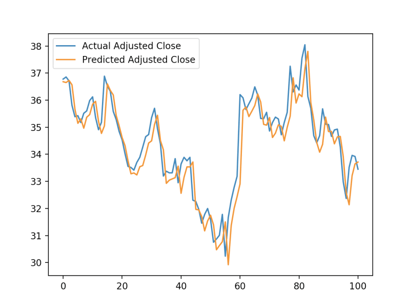
# Plot prediction vs actual
pyplot.plot(unscaled_actual_data, label='Actual Adjusted Close')
pyplot.plot(unscaled_predictions, label='Predicted Adjusted Close')
pyplot.legend()
pyplot.show()

So we see that although the error was relatively low, the model ended up learning that the best prediction for a closing price is the one closest to the previous day’s closing price.

Though these results certainly aren’t groundbreaking, it’s a pretty good start for such a basic model. With a few tweaks to the model architecture, data presentation, and variety of data sources, I believe it could generate more compelling predictions. Try it out for yourself and see how much you can improve upon what we started with here.

Inspiration

Code-free tool for modeling stock prices

If you’d rather just try your hand at generating models based on various stock market data sources, check on the Stock Modeling Tool. It does all the hard work for you. All you have to do is pick which data sources you want to input into the model and which item you want the model to predict.